Music trend (1920-2020)

Notable Trends in attributes of Spotify songs

How can we tell how music is changing? What types of music trends are happening? These are the questions for which we wanted to find answers. It would be fairly difficult analyzing music by listening to thousands (or even hundreds) of songs, but luckily for us, Spotify shares lots of data. Yamaç Eren Ay posted a data set on the website Kaggle, which included data for more than 160 thousand songs all from Spotify. This data includes songs from 1921 up to 2020, and looks at a number of different variables for each song. Our goal is to analyze how these factors have changed for music since 1921 with an emphasis on how music has been changing in the last decade.

Song Energy

The following plot is the distribution of energy songs for a decade from 1920s to 2010s. We observe that prior to the 1960s most of the songs that were realeased had low energy. The curve flattened out in the following two decades and slowing started skewing towadrs high energy. From this trend we can predict that in 2020 there will be more songs with higher energy than lower energy.

library(tidyverse)
library(plotly)
library(scales)

spotify_data <- read_csv("data.csv")


decade_detect <- function(year) (floor(year/10)*10)

get_density <- function(data) data.frame(density(data$energy)$x,density(data$energy)$y)


df <- spotify_data %>%
        filter(year<2020) %>% 
        mutate(decade=decade_detect(year)) %>%
        group_by(decade) %>% 
        nest() %>%
        mutate(dens = map(data,get_density)) %>% 
        unnest(dens)

ax <- list(title = "Energy (higher value = higher energy)",
           zeroline=FALSE,
           range = c(0,1))
ay <- list(title = "Density")

fig <- df %>%
  plot_ly(
    x = ~df$density.data.energy..x,
    y = ~df$density.data.energy..y,
    type = 'scatter',
    mode = 'lines',
    frame=~df$decade,
    showlegend = FALSE
  )
fig <- fig %>% 
          layout(xaxis = ax, yaxis = ay) %>% 
          animation_slider(
            currentvalue = list(prefix = "Decade ",
                                suffix="s",
                                font = list(color="blue"))
            )
fig

Energy vs Popularity

Given that there are more and more song that have high energy a natural assumption to make is that the these songs are more popular than the low energy songs. But this is not the case according to the data. From the following plot we can see that the popularity is constant as the energy varies. This means that lower energy songs are equally as popular as high energy one even though there are a lot of the latter being released released

df1 <- spotify_data %>% 
        filter(year>2009,year<2020)

ax <- list(title = "Energy (higher value = higher energy)",
           zeroline=FALSE,
           range = c(0,1))
ay <- list(title = "Popularity")

fig <- df1 %>%
          plot_ly(x = ~df1$energy,
                  y = ~df1$popularity,
                  type = 'scatter',
                  frame=~df1$year,
                  showlegend = FALSE
                  )

fig <- fig %>% 
          layout(xaxis = ax, yaxis = ay) %>% 
          animation_slider(
            currentvalue = list(prefix = "Year ",
                                font = list(color="blue"))
            )

fig

Remark: We can observe that the average popularity of songs go up as we go through the decades. This is because the popularity refers to current popularity and not when the song was released.

Acousticness

Consider the graph below that shows how the average acousticness of music has changed over the years. Acousticness is defined to be the chance that a track is acoustic.

library(tidyverse)
library(scales)
library(gridExtra)
data <- read_csv("data.csv")
data_by_year <- read_csv("data_by_year.csv")
data_2010s <- data %>% 
  filter(2010 <= year, year <= 2019)
data_2010s_p <- data_2010s %>% 
  slice_max(popularity, n = floor(nrow(.)/10))
data_2010s_a <- data_2010s %>% 
  slice_max(acousticness, n = floor(nrow(.)/10))
data_2010s_pa <- semi_join(data_2010s_p, data_2010s_a) %>% 
  mutate(clean_artists = str_sub(artists, 3, -3))
data_2010s_pa$year <- factor(data_2010s_pa$year, ordered = is.ordered(data_2010s_pa$year))
data_by_year %>% 
  ggplot() +
    geom_smooth(mapping = aes(x = year, y = acousticness, color = "red")) +
    labs(x = "Year",
         y = "Acousticness", 
         title = "Acousticness over time",
         subtitle = "Years 1920-2020") +  theme(legend.position = "none")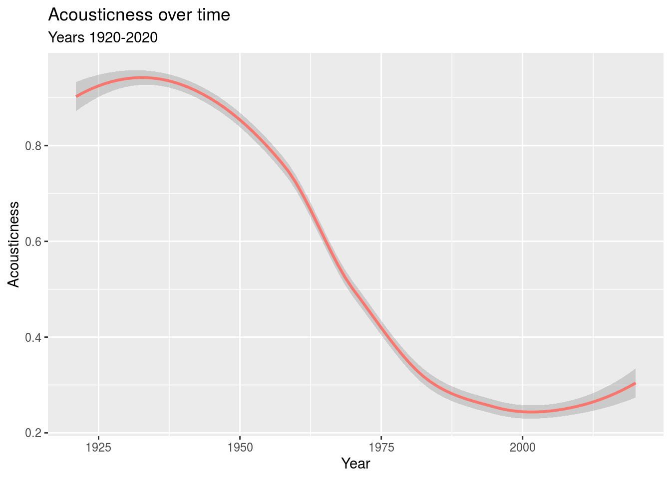

Notice that there has been a recent increase in acousticness. To investigate this further, we examined just the data for 2010-2019, the most recent complete decade. The graph below shows that the songs in the top 10% of both acousticness and popularity for this decade mostly were released late in the decade.

p1 <- data_2010s_pa %>% 
  group_by(year) %>% 
  mutate(total = n()) %>% 
  filter(total >= 3) %>% 
  ggplot() +
    geom_bar(mapping = aes(x = year, fill = (clean_artists == "Billie Eilish"))) +
    labs(x = "Year",
         y = "Number of songs", 
         title = "Number of songs in the top 10% of acousticness and popularity",
         subtitle = "Years 2010-2019",
         fill = "Year") +
    scale_fill_discrete(labels = c("Other","Billie Eilish"))


p2 <- data_by_year %>% 
  filter(year > 2009, year < 2020) %>% 
  ggplot() +
    geom_smooth(mapping = aes(x = year, y = popularity)) +
    scale_x_continuous(breaks = pretty_breaks()) +
    labs(x = "Year",
         y = "Popularity", 
         title = "Popularity over time",
         subtitle = "Years 2010-2019",
         fill = "Year")
grid.arrange(p1,p2)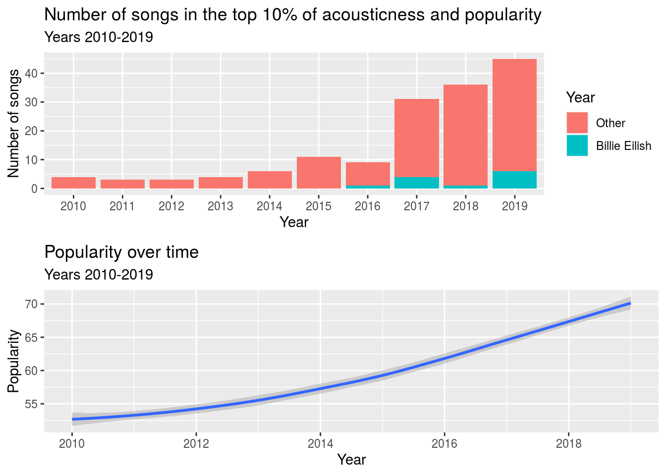

Notice that the most popular acoustic songs are concentrated toward the end of the decade, and that this concentration is higher than the general increase in popularity over time. This suggests that acoustic songs became more popular toward the end of the decade. In an effort to see what may have caused this, we noticed that the increase happened around the time that Billie Eilish started getting media attention. Billie has more than double any other artist’s popular acoustic tracks, despite only starting her career in 2016.

data_2010s_pa %>% 
  group_by(artists) %>% 
  mutate(total = n()) %>% 
  filter(total >= 3) %>%
  ggplot() +
    geom_bar(aes(x = fct_reorder(clean_artists,total), fill = (year %in% c(2017,2018,2019)))) +
    labs(x = "Artist",
         y = "Number of songs", 
         title = "Number of songs in the top 10% of acousticness and popularity",
         subtitle = "Years 2010-2019; only artists with at least 4 songs shown",
         fill = "Year") +
    scale_y_continuous(breaks = pretty_breaks()) +
    scale_fill_discrete(labels = c("Before 2017","2017 or later")) +
    coord_flip()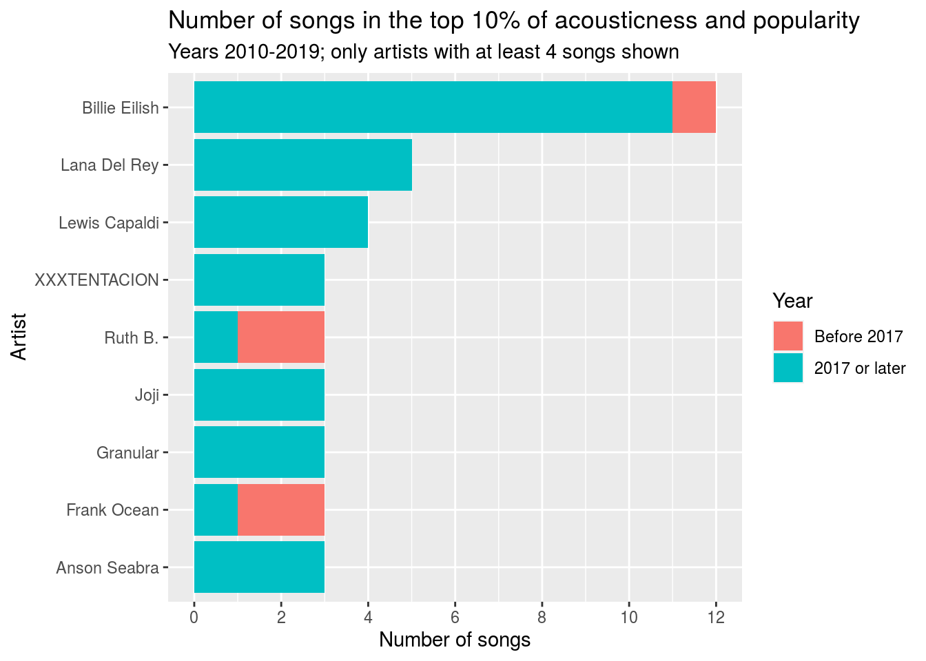

Explicit factor

Something that has become much more popular in music lately is having explicit lyrics. For example, here is a bar chart showing the percentage of explicit songs in the data by each decade.

musicdata <- read_csv("data.csv")

musicdata_2010s <- musicdata %>% 
  filter(year %in% 2010:2019) %>% 
  select(-X1, -id)

musicdata$year <- factor(musicdata$year, ordered = is.ordered(musicdata$year))
musicdata_bydecade <- musicdata
musicdata_bydecade$decade <- paste0(substr(musicdata_bydecade$year, start = 1, stop = 3),0)
musicdata_bydecade <- musicdata_bydecade %>% select(-X1)
musicdata_bydecade %>% 
  group_by(decade) %>% 
    summarise(explicit_ratio = mean(explicit))  %>% 
  ggplot() +
  geom_col(mapping = aes(x = decade, y = explicit_ratio * 100), fill = "darkblue") +
  labs(title = "Percent of Songs that are Explicit by Decade", x = "Decade", y = "Percent of Songs that are Explicit")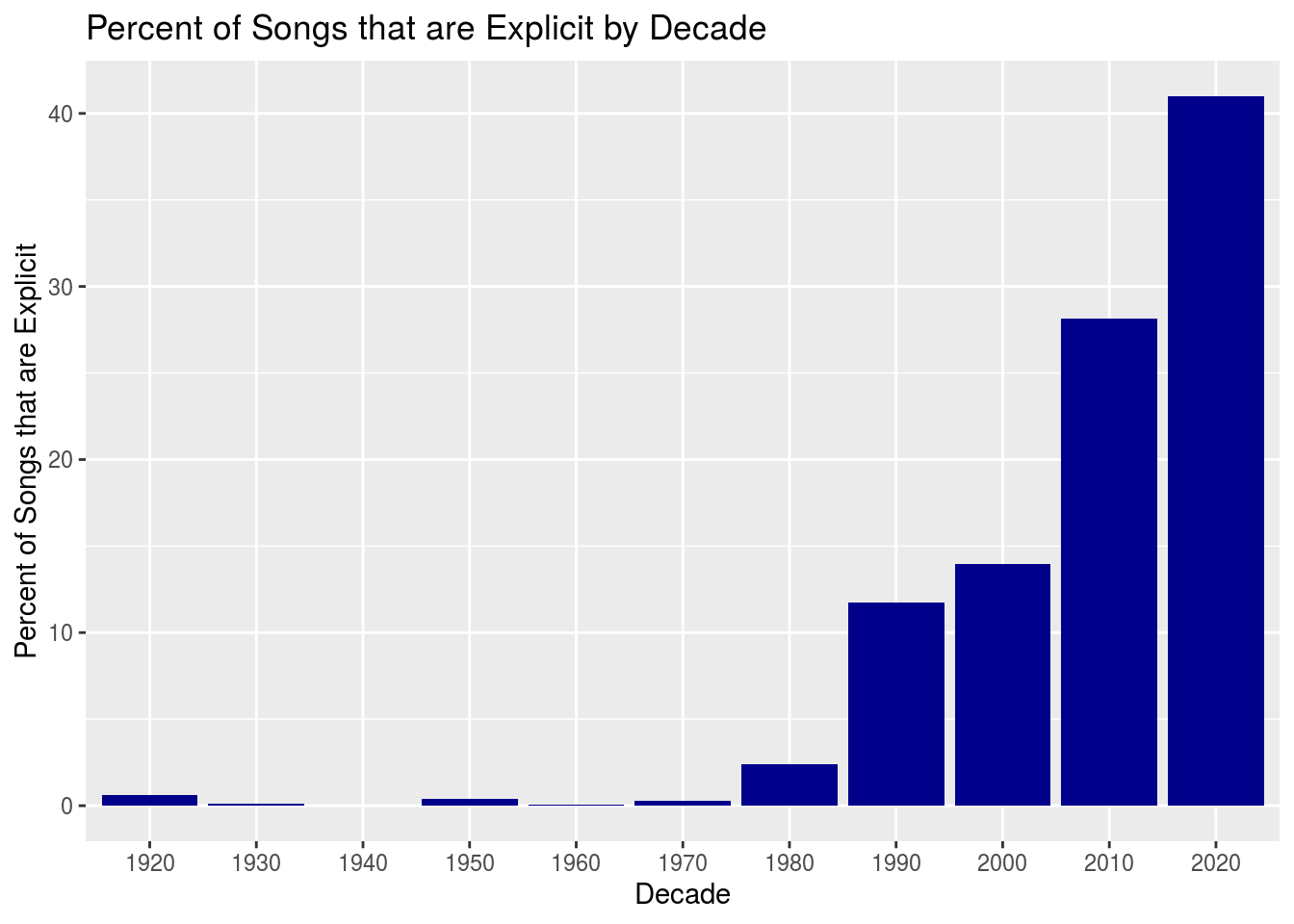

Above you can see that explicit songs were very rare, up until about the 1990s, where more than 10% of the songs were explicit. As we look at more current music, say in the 2010s, more than a quarter of the music from the data was explicit. The data shows that more than 40% of music from 2020 was explicit as well. Something to keep in mind here is that we have barely entered the 2020 decade, so there isn’t much data in this decade for us to look at.

musicdata_2010s$year <- factor(musicdata_2010s$year, levels = c("2010", "2011", "2012", "2013", "2014", "2015", "2016", "2017", "2018", "2019"))
musicdata_2010s %>% 
  group_by(year) %>% 
  summarise(explicit_ratio = mean(explicit))  %>% 
  ggplot() +
  geom_col(mapping = aes(x = year, y = explicit_ratio * 100), fill = "darkblue") +
  labs(title = "Percent of Songs that are Explicit by Year in the 2010s", x = "Year", y = "Percent of Songs that are Explicit")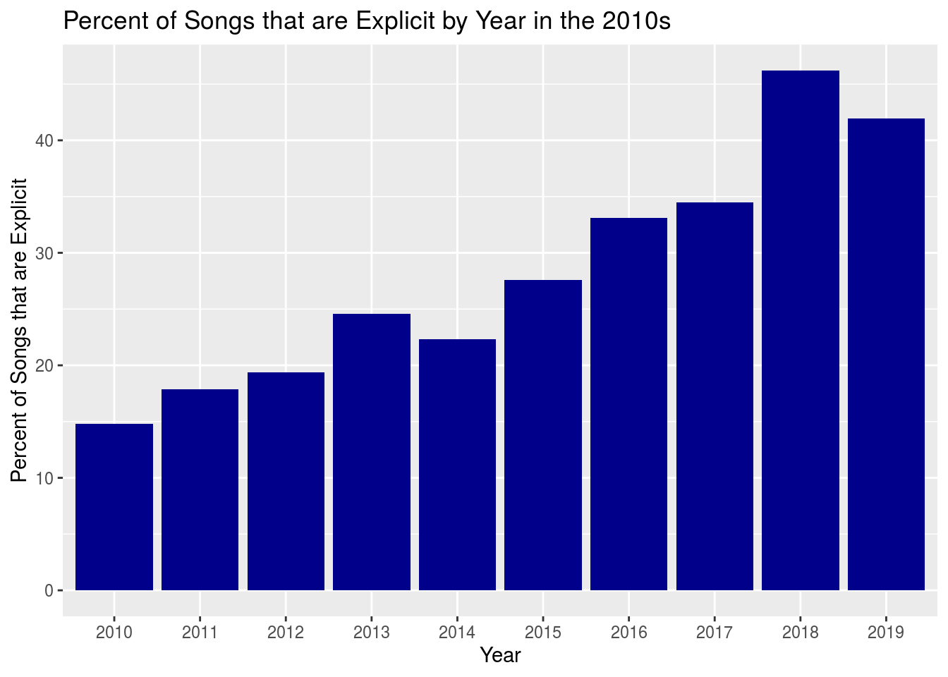

If we focus specifically on the 2010 decade, we can see that explicit songs became much more prevalent as the decade went on. Something here to notice is that there was actually a peak in 2018, where more than 45% of the songs were explicit.

musicdata$explicityn <- factor(musicdata$explicit, labels = c("0","1"))
musicdata_explicit <- musicdata %>% 
  mutate(explicityn = fct_recode(explicityn, "Yes" = "1", "No" = "0"))
musicdata_explicit %>% 
  group_by(year, explicityn) %>% 
  summarise(avg_energy = mean(energy)) %>% 
  ungroup() %>% 
  ggplot() +
  geom_line(mapping = aes(x = year, y = avg_energy, group = explicityn, color = explicityn)) +
  scale_x_discrete(breaks=seq(1920, 2020, 10)) +
  labs(title = "Average Song Energy by Year", subtitle = "Grouped by whether the song is explicit or not", x = "Year", y = "Energy", color = "Explicit")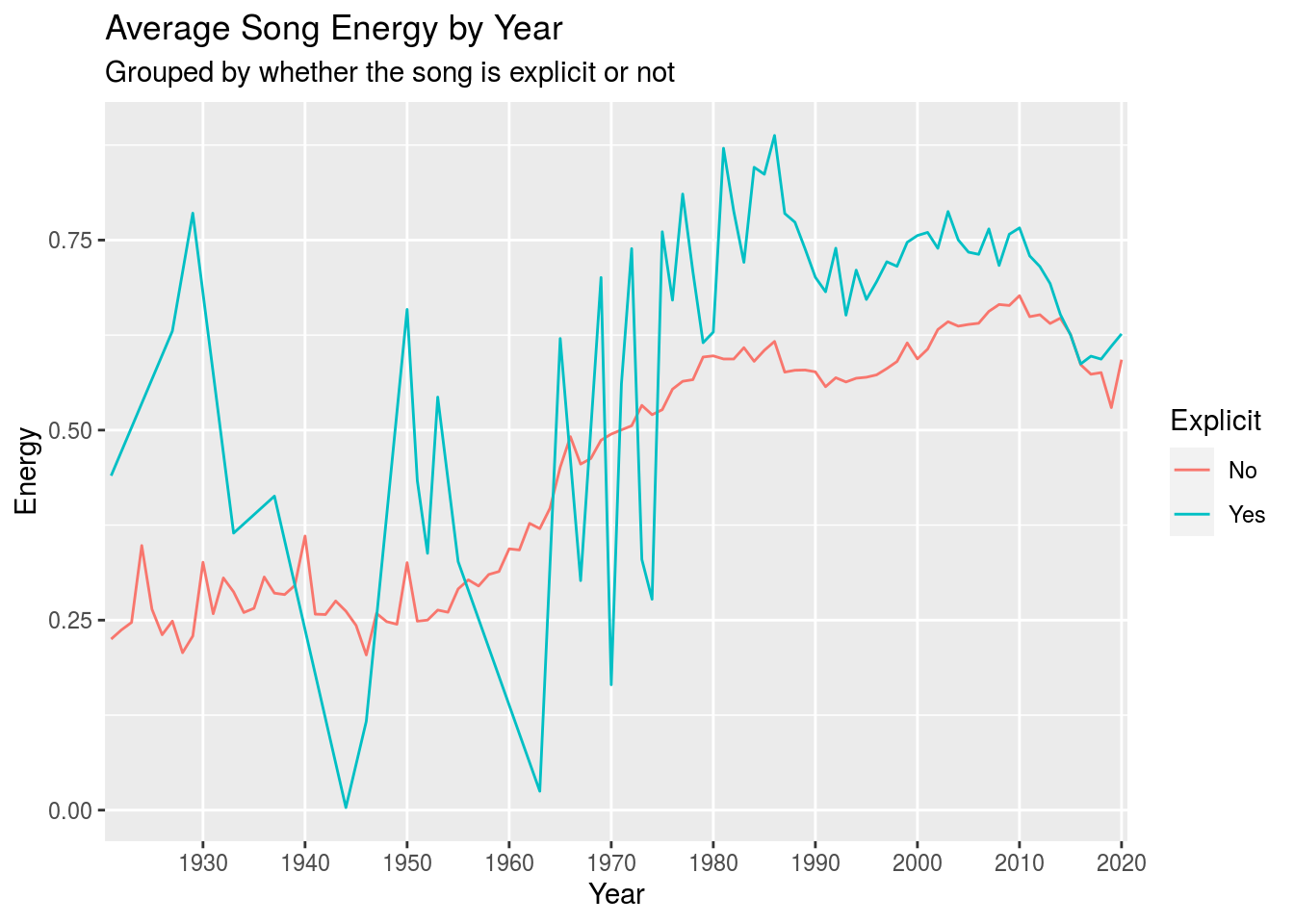

Something interesting to look at is the energy of songs throughout the years. Remember that there weren’t very many explicit songs before 1990, but after about 1975, the average energy (for each year) of explicit songs has been higher than non-explicit songs. In fact, we can even see that the energy for both explicit and non-explicit songs are tending to be much higher in the more current music.

musicdata$explicityn <- factor(musicdata$explicit, labels = c("0","1"))
musicdata_explicit <- musicdata %>% 
  mutate(explicityn = fct_recode(explicityn, "Yes" = "1", "No" = "0"))
musicdata_explicit %>% 
  group_by(year, explicityn) %>% 
  summarise(avg_pop = mean(popularity)) %>% 
  ungroup() %>% 
  ggplot() +
  geom_line(mapping = aes(x = year, y = avg_pop, group = explicityn, color = explicityn)) +
  scale_x_discrete(breaks=seq(1920, 2020, 10)) +
  labs(title = "Average Song Popularity by Year", subtitle = "Grouped by whether the song is explicit or not", x = "Year", y = "Popularity", color = "Explicit")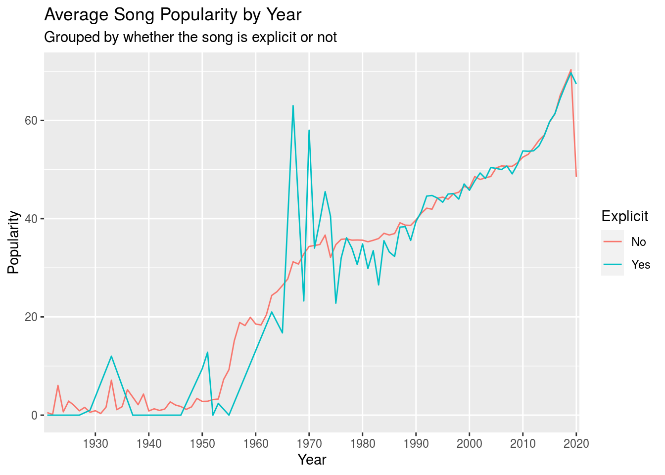

Since explicit music has become more prevalent, we can notice that a song being explicit or not does not have a large affect on the popularity of the music. One might expect that non-explicit songs would be more popular than explicit songs, since they are more “family-” or “radio-friendly”. This, however, does not seem to be the case.

Conclusion

spotify_data %>%
  group_by(year)  %>%
  summarise(acousticness = mean(acousticness), energy = mean(energy),instramentalness = mean(instrumentalness), explicit = mean(explicit)) %>%
  ggplot() +
    geom_line(mapping = aes(x=year, y=acousticness, color='acousticness')) +
    geom_line(mapping = aes(x=year, y=energy, color = 'energy')) +
    geom_line(mapping = aes(x=year, y=instramentalness, color='instramentalness')) +
    geom_line(mapping = aes(x=year, y=explicit, color = 'explicit')) +
    labs(title = 'Some Clear Trends in the Past Century of Spotify', x = 'year', y = 'value')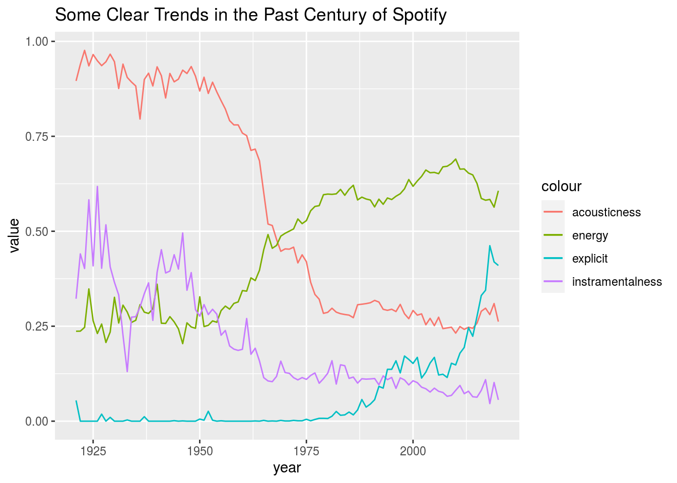

We think it would be interesting to replace popularity with (highest popularity rating) meaning the peak popularity that a song hit after being released. But even then, some debate arises amongst songs whose peak popularity sharlpy rose and declined but its popularity value was (much) higher than the peak popularity of a song that remained very popular for an extended period of time. Perhaps a combination of these two would give rise to a better popularity value for a song.

Anyways, for the average song released on Spotify, its acousticness and instramentalness saw trends as time became more and more current. They both decreased and recently have seemed to leveled off. In the next few years, the average Spotify song can expect to have an acousticness rating of ~.26 and instramentalness of ~.06

In contrast, the energy and whether or not a song was explicit both saw upwards trends as time went on for the average song released on Spotify. THe energy seems to have level off recently, whereas whether or not a song was explicit seems to have a small upwards trends. We expect it to level off. We just can’t predict exactly when or at what level, but We would guess it’ll level off within the next decade around ~33% (meaning that ~33% of the songs relseaed on Spotify each new year will contain explicit language).